

The main stress regions in a cable gland are loaded entry threads and runouts, body transitions, seal or clamp edges, the cable exit and the enclosure mounting. Which region governs depends on how force travels through the installed cable, gland and wall. I start with that load path, then use finite element analysis (FEA) to examine the parts and contacts that carry it.
A useful model answers a specific design question: whether a larger fillet reduces local strain, whether bending opens part of the seal, or whether a thin mounting panel flexes enough to disturb the joint. The required output follows that question. Metal stress, seal pressure and cable movement describe different responses.
Key takeaways
- Trace the force from the loaded cable layer through the gland into the enclosure.
- Include assembly preload before applying service loads.
- Resolve thread roots, radii and contact edges where their local response matters.
- Check cable support and wall stiffness when bending moves the hotspot.
- Compare stable numerical quantities with measurements on the same assembly.
Where should a cable-gland FEA review begin?
Finite element analysis represents geometry with small connected elements and solves their response to specified materials, loads, contacts and restraints. A stress concentration is a local rise associated with a geometric or load-transfer change. The cable entry contains several such changes, so I inspect the complete installed joint before choosing a smaller region for detailed analysis.
Follow the load from the cable layer touched by the grip or clamp. It passes through the gland body and entry connection into the enclosure and its supports. The load can cross a sliding interface, an elastomer or an armour clamp. A bonded contact assumption can suppress movement that occurs in the real joint.
| Region to inspect | Physical reason | Result that helps explain it |
|---|---|---|
| Loaded thread flanks, roots and runout | Force is shared through small profiles and changes direction | Thread load sharing, local strain and joint opening |
| Body shoulder, undercut and wall transition | Section and stiffness change | Stress/strain distribution and permanent deformation |
| Seal edge and sealing band | Assembly deformation creates contact | Pressure distribution, contact width and separation |
| Cable grip or armour clamp | Force enters a particular cable layer | Slip, layer movement and contact load |
| Cable exit | Flexible cable meets a stiff boundary | Bending strain and local cable curvature |
| Panel, washer, locknut or tapped boss | Mounting parts close the load path | Panel deflection, bearing and entry rotation |
Identify the cable construction before assigning those contacts. The armoured-versus-unarmoured comparison shows why an armour clamp and a jacket grip carry force through different layers. A screen contact used for electromagnetic compatibility (EMC) needs its separately specified mechanical role.
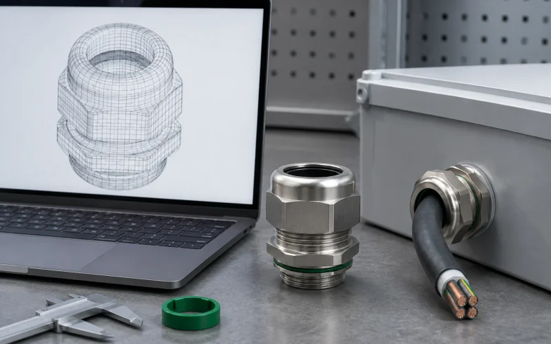
A workbench scene places a cable-gland sample, an enclosure entry, a caliper and an unlabeled wireframe model side by side.
Choose the load cases before refining the mesh
Preload is the initial force or deformation created during assembly. Tightening can establish thread contact, seat the shoulder and compress the seal before any external pull occurs. I solve or otherwise represent this assembly state first, then apply the service load sequence appropriate to the question.
Axial pull, lateral force, pressure and thermal movement can act through different paths. Vibration adds a time-dependent response; temperature can change both material behaviour and initial interference. Keep direction, load application area and the position of external supports with each case so a later variant is compared on the same basis.
| Load case | Assembly detail to retain | First response to inspect |
|---|---|---|
| Axial cable pull | Correct gripping layer and cable support | Slip and force transferred to the body |
| Exit bending | Cable stiffness, load direction and distance to entry | One-sided opening, strain and panel rotation |
| Tightening | Contact friction, closure method and tool reaction | Preload and seating at each joint |
| Internal pressure | Exposed surfaces and seal condition | Separation, extrusion and wall reaction |
| Temperature change | Component expansion and temperature-dependent properties | Changed interference and contact width |
| Repeated motion | Cycle history, restraint and relevant dynamic response | Stress/strain range and contact changes |
Worked example: compare two bending moment inputs
For a force with perpendicular distance from a reference point, its moment magnitude is . Here is in newtons, in metres and in newton-metres. NASA Glenn’s moment explanation gives this force-and-distance relationship.
Suppose two hypothetical loading arrangements each transmit an 80 N transverse force at the cable entry. In A, the force line is 100 mm from the chosen entry reference; in B, it is 40 mm away. These are deliberately selected inputs for a static comparison, rather than simulated gland performance.
| Arrangement | Perpendicular distance | Calculated moment at the reference |
|---|---|---|
| A | 0.100 m | 80 × 0.100 = 8.0 N·m |
| B | 0.040 m | 80 × 0.040 = 3.2 N·m |
I find a 60% lower moment in B from this calculation, while the transverse force remains 80 N. The model must still apply both the force and the appropriate moment when the loading is transferred to that reference point. If the actual cable route or support changes the force too, calculate the new force distribution instead of retaining this assumed value.
This comparison helps choose loading cases and support geometry. It does not supply an allowable stress or prove that a particular support spacing is suitable. Include cable bending limits, support stiffness and the joint’s actual response when selecting the installed arrangement.
Resolve the loaded thread and body transitions
Thread engagement is the overlap of mating threads that can transfer load in the seated assembly. Thread runout is where the full thread form terminates. A fillet is the rounded transition between surfaces. These features deserve local detail when the question concerns thread strain or a body-transition hotspot.
Use the installed engagement rather than the visible male projection. Panel thickness, counterbores, washers, locknuts and adapters affect which threads engage and where the shoulder seats. The M20 specification guide helps establish those dimensional inputs.
I include mating-part stiffness, friction and preload when checking load sharing. For a thin clearance-hole panel, model the shoulder, entry seal, wall and locknut contacts. For a tapped boss, model the relevant female thread and supporting material. A fully fixed cut face can make the mounting much stiffer than the installation.
At a body transition, retain the manufactured radius and wall thickness. Compare a revised fillet under the same applied loads and mounting assumptions, then check whether the change also affects seal space, tool access or thread length. A local stress improvement is useful only within a workable complete design.
Separate a stress concentration from a singularity
A stress singularity is a model location where the idealized local stress grows without a finite limit. A mathematically sharp corner or point restraint can create this behaviour. NAFEMS’ mesh-convergence guidance explains how a zero-radius internal corner produces rising stress with refinement and why the manufactured fillet radius matters.
When a peak keeps increasing, inspect its geometry and boundary condition before treating it as a physical failure prediction. Represent the real radius or load-bearing area when local stress there is the design question. For another question, define an appropriate path, area or displacement output and demonstrate its numerical stability. Keep that evaluation definition the same between variants.
Read seal contact and cable retention separately
Contact pressure is compression transmitted across an interface. For a seal, inspect where contact exists, its width and how it changes with load. Von Mises stress combines a metal stress state into a scalar often used in a ductile-yield assessment. The metal contour and seal-contact map answer different questions.
I inspect the deformed seal alongside its pressure and strain results. An edge peak with an opening elsewhere can behave differently from a continuous compressed band. Include the actual seal profile, cable diameter and shape, assembly closure and appropriate elastomer behaviour. Temperature and time-dependent relaxation may matter to the intended service state.
The seal cold-flow guide explains why contact can change after assembly. For a time-dependent question, use relevant material data and load history. Then compare the modeled contact response with the sealing function measured on the represented assembly.
At a retention interface, track relative cable movement and the layer carrying the load. A jacket may move relative to inner components; an armoured design introduces its own clamp and preparation dimensions. The sealing and strain-relief guide helps separate external cable support, gripping and environmental sealing.
Build a model that preserves the important interfaces
I specify the model at the level needed for its intended decision. A global model can establish panel movement and reactions; a detailed local model can examine a thread root or fillet using a consistent transferred boundary condition. The geometry omitted from either model must remain compatible with the response being investigated.
NASA-STD-7009B links modeling practice to intended use and defined acceptance criteria for NASA activities. Applied as a modeling principle here, this means agreeing on the question and useful comparison before the result is plotted. For a cable-entry study, agree on the required output and comparison criterion before evaluating the variants.
Record the following inputs with each model revision:
- Assembly: gland variant, cable layers, entry, accessories and drawing revisions.
- Geometry: tolerances, radii, wall thickness and simplifications relevant to the question.
- Materials: metal and elastomer models, temperature, conditioning and data ranges.
- Contacts: bonded, separating or sliding behaviour, friction and interference.
- Assembly state: seating, preload and seal closure before service loading.
- Loads and restraints: magnitude, direction, area, sequence and actual fixture or enclosure support.
- Outputs: quantity, location, averaging, units and the criterion for comparison.

Check equilibrium, mesh sensitivity and model assumptions
Start with the deformed shape and reactions. Unexpected rigid movement points toward missing restraint. A body that barely moves while the test panel flexes suggests that the support representation needs attention. Confirm that the applied forces and moments balance the reactions for a static equilibrium case.
For example, if a hypothetical static model applies 200 N in one direction and reports only 170 N of total opposing reaction, 30 N remains unexplained. That is 15% of the applied load. Check whether the export omitted a support or other force contribution, whether the load step has converged and whether the intended case is actually static. Resolve the balance before using its stress plot to compare designs.
Mesh sensitivity describes how the selected result changes as the discretization is refined. Refine the relevant region and compare the same quantity at the same physical location. Use a defined convergence criterion appropriate to the decision. A stable average displacement does not automatically establish that a local contact-pressure peak is resolved.
Sensitivity analysis examines how outputs change when inputs or assumptions vary. I vary uncertain friction, cable stiffness, material properties or mounting restraint within justified ranges. If the preferred design changes across plausible inputs, focus measurements on the input controlling that choice. This identifies where additional physical information is useful.
The NASA-HDBK-7009A glossary and guidance distinguish verification, empirical validation, sensitivity and uncertainty. Verification checks implementation and numerical solution. Validation compares the model with the physical system for the intended use. Mesh refinement supports the numerical check; matched measurements address the physical comparison.
Compare each predicted response with a useful measurement
Select measurements that observe the same load path as the model. A load cell can check the applied force, a displacement measurement can track panel or gland movement, and suitable strain measurements can compare accessible body regions. Record sensor position and direction so the simulation output can be evaluated at the corresponding location.

| Modeling question | Physical comparison | Design information gained |
|---|---|---|
| Does the entry or body deform under load? | Load, displacement, strain and permanent-set inspection | Local stiffness and load distribution |
| Does bending disturb the seal? | Assembly movement, leakage and post-test seal condition | Contact changes and sealing response |
| Does the cable slip or suffer layer damage? | Pull or torsion loading with cable movement recorded | Retention path and slip onset |
| Does the panel govern movement? | Panel deflection and mounting contact marks | Effect of wall and fixture stiffness |
| Where does repeated loading cause damage? | Defined cyclic exposure and planned inspections | Relevant location and load-history response |
ASME V&V 10-2019 (R2025) provides a framework for verification, validation and uncertainty in computational solid mechanics. I use the comparison to identify which model inputs need correction and how well the result supports the stated design decision.
IEC 62444:2010 covers requirements and tests for complete cable glands within its scope. Apply the relevant product tests and installed conditions alongside the analysis. A static stress result addresses its modeled load case; ingress, retention and cyclic durability each need the assessment appropriate to that function.
Turn the hotspot into a design decision
Choose the change that addresses the physical cause. A body-transition concentration can prompt a radius or section review. Uneven seal contact can prompt changes to the profile, closure or cable fit. Entry rotation can prompt a mounting or panel-stiffness review, while exit bending can prompt a cable-route or support change.
I compare each revision using the same output definition and service question. Keep the revised assembly state consistent, and recheck adjacent interfaces affected by the change. For example, a larger shoulder may improve mounting stiffness while reducing tool clearance, and a changed seal cavity may alter closure loads on the body.
Conclusion
The critical region in a cable gland follows the load path through its cable contact, body, entry and enclosure. Start with the installed geometry and assembly state, then examine the local thread, transition, seal or exit response for each relevant load case.
I use equilibrium checks, stable output definitions and physical comparisons to turn an FEA hotspot into a useful design change. The bending example shows why loading geometry matters before meshing begins; the reaction example shows why a plausible contour needs a balanced mechanical model behind it.
FAQs about cable-gland FEA stress points
Are cable-gland thread roots always the highest-stress location?
Loaded roots and runouts are important review locations. Cable bending, body transitions, seal contact or panel flexibility can make another region govern. Trace the actual force path and compare the relevant stress, contact and movement outputs for the installed assembly and load case.
Does a red FEA contour mean the cable gland will fail there?
Red identifies the upper end of the displayed scale. Check the result quantity, units, load step and material criterion, then examine numerical stability at that location. A singular corner peak needs a different interpretation from a resolved stress concentration in the manufactured geometry.
How can FEA support a cable-gland service-life estimate?
It can supply stress or strain histories for defined loads and cycles. A life estimate also needs suitable durability data, the service load history, environmental effects and an applicable damage model. Compare the resulting prediction with relevant physical observations before using it for a maintenance decision.
How should brass, stainless-steel and polymer gland designs be compared?
Use the same service question while giving each design its actual geometry, contacts, assembly state and material behaviour. Evaluate metal, polymer and seal responses with appropriate criteria. Check temperature and time-dependent behaviour where relevant, then compare the complete assemblies through suitable measurements and tests.
Sources and technical references
- NASA-STD-7009B — Standard for Models and Simulations, accessed 2026-10-29.
- ASME V&V 10-2019 (R2025) — Verification and validation in computational solid mechanics, accessed 2026-10-29.
- NASA-HDBK-7009A — Handbook for Models and Simulations, accessed 2026-10-29.
- IEC 62444:2010 — Cable glands for electrical installations, accessed 2026-10-29.
- NAFEMS — The importance of mesh convergence, accessed 2026-10-29.
- NASA Glenn — Moment and equilibrium explanation, accessed 2026-10-29.