# 並聯導體：檢查電流密度與分流不均

> Source: https://chinacableglands.com/zh-hant/blog/current-density-parallel-conductor-resistance/
> Language: zh-Hant
> Publisher: 倍拓電纜接頭
> Author: Victor Huang
> Published: 2026-10-22
> Updated: 2026-10-23

使用金屬導體截面積比較電流密度，並以明確界定的相同路徑計算並聯電阻；同時將載流量、電流分配及端子核准分開判斷。

<p><strong>電流密度是以導體截面積為基礎比較電流；並聯電阻計算則比較電氣路徑。單靠這兩種計算，都無法確定電纜載流量或允許導體並聯使用。</strong>若要將模型用於規劃中的配置，必須先確認實際導體、電路條件及設計依據。</p>
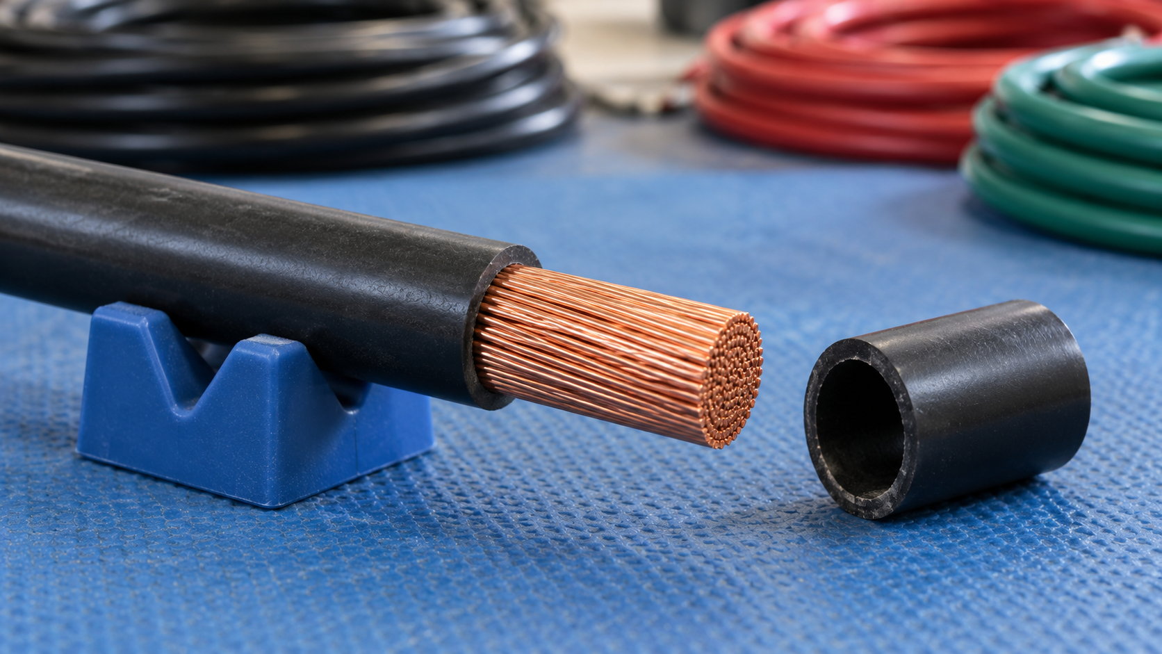
<p>這項區分對電纜引入口也很重要。電氣計算使用金屬導體截面積，而電纜密封接頭或後端密封件使用完成品電纜直徑。不能把整條有絕緣層的電纜視為實心導體，從而以其中一個量值推算另一個。</p>
<h2 id="define-the-conductor-area-and-current-first">先界定導體截面積與電流</h2>
<p>在理想的均勻電流分布下，平均電流密度為：</p>
<div class="article-math article-math-display" data-latex="J=\frac{I}{A}"><span class="katex"><math xmlns="http://www.w3.org/1998/Math/MathML" display="block"><semantics><mrow><mi>J</mi><mo>=</mo><mfrac><mi>I</mi><mi>A</mi></mfrac></mrow><annotation encoding="application/x-tex">J=\frac{I}{A}</annotation></semantics></math></span></div>
<p>電流 <span class="article-math article-math-inline" data-latex="I"><span class="katex"><math xmlns="http://www.w3.org/1998/Math/MathML"><semantics><mrow><mi>I</mi></mrow><annotation encoding="application/x-tex">I</annotation></semantics></math></span></span> 以安培表示，金屬導體截面積 <span class="article-math article-math-inline" data-latex="A"><span class="katex"><math xmlns="http://www.w3.org/1998/Math/MathML"><semantics><mrow><mi>A</mi></mrow><annotation encoding="application/x-tex">A</annotation></semantics></math></span></span> 以 mm² 表示，所得電流密度單位為 A/mm²。面積不包括絕緣層、外被、絞線間的空隙及其他非導電部分。電纜含有多條電路導體時，也不能自動將其截面積相加，視為一條電流路徑可用的面積。</p>
<p>請記錄面積是規定的標稱導體尺寸，還是實測的金屬截面積。<a href="https://webstore.iec.ch/en/publication/71891">IEC 60228:2023</a> 在其適用範圍內規定了標稱導體截面積，以及結構與電阻要求。標稱尺寸是依這些要求使用的代稱，不應被描述成特定試樣的精密測量值。</p>
<p>若電流為 24 A，規定面積為 4 mm²，平均電流密度為 6 A/mm²。若輸入 8 mm²，計算結果為 3 A/mm²。這項比較呈現以面積正規化後的電流值，不會考慮散熱、絕緣溫度、成束、安裝方式或導線端接處的接點。</p>
<p>也必須明確說明電流條件。直流計算、用於熱比較的 RMS 電流，以及瞬態峰值，各有不同用途。在頻率或導體尺寸會造成電流分布不均的情況下，這項簡單平均值無法描述局部電流分布。</p>
<figure>
<img src="/images/blog/current-density-parallel-conductor-resistance/current-density-parallel-conductor-resistance-scene-01.png" alt="已剝除絕緣層的絞合銅導體放在藍色工作墊上，旁邊另有一段獨立的中空黑色絕緣材料" width="1672" height="941" loading="lazy" decoding="async">
<figcaption>裸露的銅線束與取下的絕緣層，分別呈現導體金屬與整體絕緣電纜直徑。</figcaption>
</figure>
<h2 id="compare-with-an-entered-density-basis">與輸入的電流密度依據比較</h2>
<p>電流密度計算器可顯示結果與輸入專案限值之間的餘裕。若將示例結果 6 A/mm² 與獨立提供的 7.5 A/mm² 依據比較，計算餘裕為 1.5 A/mm²，使用率為 80%。</p>
<p>我會在比較資料旁記錄 7.5 A/mm² 的來源。這裡只是輸入的假設範例，不是通用建議。相較於未有文件依據的數值，即使得到正餘裕，也不能證明電纜會維持在允許溫度範圍內。</p>
<p>比較兩個候選導體時，應使用相同的電流條件與適用的比較依據。如果依據會隨導體結構或安裝方式改變，請明確記錄該變更。否則整齊的比較表可能掩蓋彼此不相容的假設。</p>
<h2 id="apply-a-specified-retained-fraction-once">指定保留比例只套用一次</h2>
<p>本網站的初步載流量模型會將截面積乘上提供的設計電流密度及保留比例：</p>
<div class="article-math article-math-display" data-latex="I_{\mathrm{base}}=A J_d,\qquad I_{\mathrm{prelim}}=A J_d\eta"><span class="katex"><math xmlns="http://www.w3.org/1998/Math/MathML" display="block"><semantics><mrow><msub><mi>I</mi><mrow><mi mathvariant="normal">b</mi><mi mathvariant="normal">a</mi><mi mathvariant="normal">s</mi><mi mathvariant="normal">e</mi></mrow></msub><mo>=</mo><mi>A</mi><msub><mi>J</mi><mi>d</mi></msub><mo separator="true">,</mo><mspace width="2em"/><msub><mi>I</mi><mrow><mi mathvariant="normal">p</mi><mi mathvariant="normal">r</mi><mi mathvariant="normal">e</mi><mi mathvariant="normal">l</mi><mi mathvariant="normal">i</mi><mi mathvariant="normal">m</mi></mrow></msub><mo>=</mo><mi>A</mi><msub><mi>J</mi><mi>d</mi></msub><mi>η</mi></mrow><annotation encoding="application/x-tex">I_{\mathrm{base}}=A J_d,\qquad I_{\mathrm{prelim}}=A J_d\eta</annotation></semantics></math></span></div>
<p>此處的 <span class="article-math article-math-inline" data-latex="J_d"><span class="katex"><math xmlns="http://www.w3.org/1998/Math/MathML"><semantics><mrow><msub><mi>J</mi><mi>d</mi></msub></mrow><annotation encoding="application/x-tex">J_d</annotation></semantics></math></span></span> 是所述的設計電流密度，<span class="article-math article-math-inline" data-latex="\eta"><span class="katex"><math xmlns="http://www.w3.org/1998/Math/MathML"><semantics><mrow><mi>η</mi></mrow><annotation encoding="application/x-tex">\eta</annotation></semantics></math></span></span> 是指定修正後保留的比例。假設面積為 6 mm²、提供的設計依據為 5 A/mm²，且保留比例為 80%，則調整前的結果為 30 A，調整後為 24 A。</p>
<p>「保留 80%」與「減少 80%」是不同指示。前者使用 <span class="article-math article-math-inline" data-latex="\eta=0.8"><span class="katex"><math xmlns="http://www.w3.org/1998/Math/MathML"><semantics><mrow><mi>η</mi><mo>=</mo><mn>0.8</mn></mrow><annotation encoding="application/x-tex">\eta=0.8</annotation></semantics></math></span></span>；後者則只保留 20%。輸入百分比前，應先釐清指示的文字。</p>
<p>請確認設計電流密度是否已包含相關的熱修正或成束修正。第二次套用相同修正會使比較失真。多個修正係數應依規範方法所要求的方式組合，不應把不同文件中方便取得的百分比任意相乘。</p>
<p>當權威的專案依據提供相關輸入值時，此模型便有用。僅憑截面積無法建立該依據。<a href="/zh-hant/blog/a-guide-to-selecting-the-correct-wire-gauge-for-sealed-connectors/">線徑選用指南</a>說明電路、接點及密封方面各自需要的決策。</p>
<h2 id="calculate-ideal-resistance-for-identical-parallel-paths">計算相同並聯路徑的理想電阻</h2>
<p>對於 <span class="article-math article-math-inline" data-latex="n"><span class="katex"><math xmlns="http://www.w3.org/1998/Math/MathML"><semantics><mrow><mi>n</mi></mrow><annotation encoding="application/x-tex">n</annotation></semantics></math></span></span> 條電阻值均為 <span class="article-math article-math-inline" data-latex="R"><span class="katex"><math xmlns="http://www.w3.org/1998/Math/MathML"><semantics><mrow><mi>R</mi></mrow><annotation encoding="application/x-tex">R</annotation></semantics></math></span></span> 的相同電阻路徑，且各路徑連接在相同兩個節點之間：</p>
<div class="article-math article-math-display" data-latex="R_{\mathrm{eq}}=\frac{R}{n},\qquad I_{\mathrm{each}}=\frac{I_{\mathrm{total}}}{n}"><span class="katex"><math xmlns="http://www.w3.org/1998/Math/MathML" display="block"><semantics><mrow><msub><mi>R</mi><mrow><mi mathvariant="normal">e</mi><mi mathvariant="normal">q</mi></mrow></msub><mo>=</mo><mfrac><mi>R</mi><mi>n</mi></mfrac><mo separator="true">,</mo><mspace width="2em"/><msub><mi>I</mi><mrow><mi mathvariant="normal">e</mi><mi mathvariant="normal">a</mi><mi mathvariant="normal">c</mi><mi mathvariant="normal">h</mi></mrow></msub><mo>=</mo><mfrac><msub><mi>I</mi><mrow><mi mathvariant="normal">t</mi><mi mathvariant="normal">o</mi><mi mathvariant="normal">t</mi><mi mathvariant="normal">a</mi><mi mathvariant="normal">l</mi></mrow></msub><mi>n</mi></mfrac></mrow><annotation encoding="application/x-tex">R_{\mathrm{eq}}=\frac{R}{n},\qquad I_{\mathrm{each}}=\frac{I_{\mathrm{total}}}{n}</annotation></semantics></math></span></div>
<p>路徑數必須是正整數。各支路電阻相同且兩端電壓相同，才會平均分流。<a href="https://learninglab.rmit.edu.au/physics/electricity/parallel-circuits/">RMIT University 並聯電路指南</a>說明了這項並聯電路關係。我們可以將其用於明確界定的理想導體路徑模型。</p>
<p>在此範例中，每條路徑的電阻為 0.060 Ω，三條相同路徑的總電流為 30 A。等效電阻為 0.020 Ω，每條路徑各承載 10 A，共同壓降為 0.60 V。請維持一致的電阻界定範圍：單程導體電阻不會自動等同於包含去程與回程的完整電路電阻。</p>
<p><a class="article-tool-card article-tool-card-link" href="/zh-hant/resource-center/tools/parallel-conductor-resistance-calculator/" aria-label="並聯導體電阻計算器"><span class="article-tool-card-index">工具</span><span class="article-tool-card-kicker">電氣導通</span><strong class="article-tool-card-title">並聯導體電阻計算器</strong><span class="article-tool-card-copy">輸入一條完整且已界定路徑的電阻、相同並聯路徑數（整數）及總電流。均流為一項假設；請另外確認實際允許的結構及各支路阻抗。</span><span class="article-tool-card-formula">Req = R1 / n</span><span class="article-tool-card-inputs" aria-label="計算器輸入項目"><em>單一導體電阻</em><em>並聯導體數</em><em>總電流</em></span><span class="article-tool-card-action">開啟計算器 <span aria-hidden="true">-&gt;</span></span></a></p><p>此處「相同」包括所選界定範圍內的材料、截面積、長度、溫度與端接貢獻。均勻導體關係式 <span class="article-math article-math-inline" data-latex="R=\rho L/A"><span class="katex"><math xmlns="http://www.w3.org/1998/Math/MathML"><semantics><mrow><mi>R</mi><mo>=</mo><mi>ρ</mi><mi>L</mi><mi mathvariant="normal">/</mi><mi>A</mi></mrow><annotation encoding="application/x-tex">R=\rho L/A</annotation></semantics></math></span></span> 說明長度、截面積及材料為何重要；NBS《<a href="https://nvlpubs.nist.gov/nistpubs/Legacy/hb/nbshandbook100.pdf">銅線表</a>》介紹了這項關係與電阻隨溫度變化的情況。與理想實心截面計算相比，實際電纜電阻資料可能更有用。</p>
<h2 id="show-what-unequal-branches-do-to-current-sharing">呈現支路不相等時的電流分配</h2>
<p>兩條路徑看起來相似，也不代表電流一定平均分配。對電壓相同的電阻支路：</p>
<div class="article-math article-math-display" data-latex="\frac{1}{R_{\mathrm{eq}}}=\frac{1}{R_1}+\frac{1}{R_2},\qquad I_1=\frac{V}{R_1},\qquad I_2=\frac{V}{R_2}"><span class="katex"><math xmlns="http://www.w3.org/1998/Math/MathML" display="block"><semantics><mrow><mfrac><mn>1</mn><msub><mi>R</mi><mrow><mi mathvariant="normal">e</mi><mi mathvariant="normal">q</mi></mrow></msub></mfrac><mo>=</mo><mfrac><mn>1</mn><msub><mi>R</mi><mn>1</mn></msub></mfrac><mo>+</mo><mfrac><mn>1</mn><msub><mi>R</mi><mn>2</mn></msub></mfrac><mo separator="true">,</mo><mspace width="2em"/><msub><mi>I</mi><mn>1</mn></msub><mo>=</mo><mfrac><mi>V</mi><msub><mi>R</mi><mn>1</mn></msub></mfrac><mo separator="true">,</mo><mspace width="2em"/><msub><mi>I</mi><mn>2</mn></msub><mo>=</mo><mfrac><mi>V</mi><msub><mi>R</mi><mn>2</mn></msub></mfrac></mrow><annotation encoding="application/x-tex">\frac{1}{R_{\mathrm{eq}}}=\frac{1}{R_1}+\frac{1}{R_2},\qquad I_1=\frac{V}{R_1},\qquad I_2=\frac{V}{R_2}</annotation></semantics></math></span></div>
<p>考慮兩條假設路徑，其電阻分別為 0.020 Ω 與 0.030 Ω，總電流為 30 A。等效電阻為 0.012 Ω，因此共同壓降為 0.36 V。較低電阻的路徑承載 18 A，另一條承載 12 A。若假設各承載 15 A，就會低估負荷較高的支路。</p>
<figure class="blog-chart">
<svg xmlns="http://www.w3.org/2000/svg" viewBox="0 0 520 500" role="img" aria-labelledby="parallel-share-title parallel-share-desc" style="font-family:var(--font-body)">
<title id="parallel-share-title">電阻不相等會造成電流分配不均</title>
<desc id="parallel-share-desc">兩條電阻路徑連接在相同兩個節點之間。在這個假設範例中，20 毫歐姆路徑承載 18 安培，30 毫歐姆路徑承載 12 安培；兩條路徑的壓降都是 0.36 伏特，總電流為 30 安培。</desc>
<text x="260" y="46" text-anchor="middle" fill="var(--color-carbon)" font-size="30" font-weight="700">電阻不相等</text>
<text x="260" y="82" text-anchor="middle" fill="var(--color-graphite)" font-size="22">兩條路徑兩端電壓相同</text>
<path d="M70 190V325M450 190V325M30 258H70M450 258H490" fill="none" stroke="var(--color-carbon)" stroke-width="3"/>
<path d="M70 190H180M340 190H450" stroke="var(--color-primary)" stroke-width="4"/>
<rect x="180" y="170" width="160" height="40" fill="var(--surface-card)" stroke="var(--color-primary)" stroke-width="3"/>
<text x="260" y="148" text-anchor="middle" fill="var(--color-carbon)" font-size="24" font-weight="700">20 mΩ → 18 A</text>
<path d="M70 325H180M340 325H450" stroke="var(--color-primary)" stroke-width="4"/>
<rect x="180" y="305" width="160" height="40" fill="var(--surface-card)" stroke="var(--color-primary)" stroke-width="3"/>
<text x="260" y="283" text-anchor="middle" fill="var(--color-carbon)" font-size="24" font-weight="700">30 mΩ → 12 A</text>
<circle cx="70" cy="258" r="5" fill="var(--color-carbon)"/>
<circle cx="450" cy="258" r="5" fill="var(--color-carbon)"/>
<text x="260" y="411" text-anchor="middle" fill="var(--color-carbon)" font-size="22">總電流：30 A</text>
<text x="260" y="453" text-anchor="middle" fill="var(--color-graphite)" font-size="22">共同壓降：0.36 V</text>
</svg>
<figcaption>兩條電阻不同的路徑會依各自電阻分配假設的總電流，但兩端壓降相同。</figcaption>
</figure>
<p>這是電路模型，不是端子接線方案。我會檢查實際導體及連接，確認長度、截面積、接觸電阻與溫度是否不相同。交流系統中，阻抗及配置也可能和直流電阻同樣重要。相同路徑計算器不會模擬這些差異。</p>
<p>並聯電纜路徑與光伏電源串列並聯也是不同概念。光伏陣列的電源電流、保護與連接器規則，不應以以上理想導體分流模型取代。電纜及接點的分布式損耗，則可參考<a href="/zh-hant/blog/calculating-voltage-drop-in-solar-arrays-and-the-impact-of-connector-resistance/">電壓降指南</a>，其中明確界定了電阻計算範圍。</p>
<h2 id="complete-the-thermal-and-protection-decisions-separately">分別完成熱設計與保護決策</h2>
<p>初步算術估算應配合採用的電氣設計方法使用，不能取代該方法。<a href="https://webstore.iec.ch/en/publication/68118">IEC 60287-1-1:2023</a> 涵蓋其所述穩態條件下的電纜載流量計算，並要求提供結構與環境參數。其適用範圍說明了為何單一電流密度數值不足以完成判斷。</p>
<p>端接也有自身的電流及溫度限制。<a href="https://webstore.iec.ch/en/publication/2399">IEC 60512-5-2:2002</a> 說明機電元件，特別是連接器的電流—溫度降額測試。導體比較無法確定連接器經測試的載流能力，也無法確定其端子是否允許接入多條導體。</p>
<p>規劃中的配置涉及以下不同問題：</p>
<table>
<thead>
<tr>
<th>決策項目</th>
<th>除以上公式外所需的佐證</th>
</tr>
</thead>
<tbody>
<tr>
<td>電纜載流量</td>
<td>採用的方法、結構、散熱、環境溫度及成束條件</td>
</tr>
<tr>
<td>並聯運轉</td>
<td>適用的佈線規則、允許的結構及實際支路分流</td>
</tr>
<tr>
<td>故障保護</td>
<td>保護協調及相關故障條件</td>
</tr>
<tr>
<td>端接</td>
<td>確切接點或端子、導體規格範圍、導體數量及處理方式</td>
</tr>
<tr>
<td>電纜引入口</td>
<td>完成品電纜外徑、電纜密封接頭範圍、支撐及外殼幾何形狀</td>
</tr>
</tbody>
</table>
<p>在總電流固定時，較低的等效電阻可以降低壓降，但不會自動使允許電流加倍，也不會授權採用新的組件配置。選擇配置之前，應將此優點與完整的熱設計、保護及介面要求一併比較。</p>
<h2 id="conclusion">結論</h2>
<p>當截面積、電流條件及比較依據都明確時，電流密度是有用的正規化比較值。提供的設計電流密度與保留比例可用於初步估算；相同的並聯路徑則可建立簡單的電阻與電流分配模型。每個結果都必須連同其計算假設記錄。</p>
<p>關鍵檢查仍包括實際電纜載流量、允許的並聯配置、支路行為及端接能力。可以利用算術找出不相等的路徑或錯誤的分母，但不能據此核准整個電路。在外殼處，還應另外核對實際電纜直徑及引入口幾何形狀，並與金屬導體截面積分開處理。</p>
<h2 id="faqs-about-current-density-and-parallel-conductors">電流密度與並聯導體常見問題</h2>
<h3 id="is-current-density-the-same-as-cable-ampacity">電流密度等同於電纜載流量嗎？</h3>
<p>不等同。電流密度是以電流除以導體截面積所得的比較值。載流量或允許電流取決於適用的設計方法，以及電纜結構、絕緣溫度、散熱、成束與安裝等條件。我只會在設計依據明確時使用電流密度比較；該結果本身不能確定允許的電路電流。</p>
<h3 id="does-doubling-conductor-area-always-double-the-permitted-current">導體截面積加倍，允許電流就一定加倍嗎？</h3>
<p>不一定。截面積變化會改變電流密度計算中的面積，通常也會改變電阻，但載流量仍由熱行為與安裝條件決定。較大的導體也必須適配確切的接點、端子及電纜引入口配置。單純按面積倍增不是完整的尺寸選用方法。</p>
<h3 id="when-can-i-divide-one-conductor-resistance-by-the-number-of-paths">何時可以將單一導體電阻除以並聯路徑數？</h3>
<p>只有在各路徑於已界定的電阻範圍內完全相同，且連接在相同兩個節點之間時才可以。均流也假設各支路條件相同。我會檢查長度、材料、截面積、溫度及端接。此計算本身不會授權導體並聯使用，也不會授權將多條導體接入同一端子。</p>
<h3 id="does-an-80-derating-entry-mean-that-current-is-reduced-by-80">降額計算器輸入 80% 是否表示電流減少 80%？</h3>
<p>如果計算器要求輸入保留比例，就不是。保留 80% 會留下未調整結果的五分之四，也就是減少 20%。我會一併核對輸入標籤與來源指示，並確認設計依據尚未包含該修正，再套用此比例。</p>
<h3 id="sources-and-technical-references">來源與技術參考資料</h3>
<ul>
<li><a href="https://webstore.iec.ch/en/publication/71891">IEC 60228:2023 — 絕緣電纜用導體</a>，查閱日期：2026-10-22。</li>
<li><a href="https://learninglab.rmit.edu.au/physics/electricity/parallel-circuits/">RMIT University — 並聯電路</a>，查閱日期：2026-10-22。</li>
<li><a href="https://nvlpubs.nist.gov/nistpubs/Legacy/hb/nbshandbook100.pdf">NBS Handbook 100 —《銅線表》</a>，查閱日期：2026-10-22。</li>
<li><a href="https://webstore.iec.ch/en/publication/68118">IEC 60287-1-1:2023 — 電纜，載流量計算</a>，查閱日期：2026-10-22。</li>
<li><a href="https://webstore.iec.ch/en/publication/2399">IEC 60512-5-2:2002 — 載流能力測試：電流—溫度降額</a>，查閱日期：2026-10-22。</li>
</ul>
