# 威布爾可靠度：如何解讀 B10 與電纜引入口壽命宣稱

> Source: https://chinacableglands.com/zh-hant/blog/weibull-cable-entry-reliability/
> Language: zh-Hant
> Publisher: 倍拓電纜接頭
> Author: Victor Huang
> Published: 2026-10-22
> Updated: 2026-10-29

閱讀威布爾可靠度、B10 與特徵壽命，透過範例、設限觀測、信賴界限及電纜引入試驗條件進行解讀。

<p><strong>威布爾可靠度描述失效機率如何隨暴露時間變化。B10 是該模型累積失效機率達 10% 時的時間；特徵壽命則是累積失效機率約達 63.2% 的時間。</strong>我會在用電纜引入口壽命宣稱作決策前，比較所述壽命指標、試驗條件及信賴界限。</p>
<p>這項差異很重要。兩個模型可以有相同的特徵壽命，但 B10 值相差很大。長時間試驗中只有少數失效，與收到大量退回零件所提供的資訊也不同。解讀曲線時，應同時查看母體以及用來配適模型的紀錄。</p>
<blockquote>
<p><strong>重點摘要</strong></p>
<ul>
<li>B10 描述模型壽命分布的早期百分位；它不同於平均壽命或特徵壽命。</li>
<li>形狀參數會改變失效率趨勢，尺度參數則決定特徵時間。</li>
<li>將仍存活試樣的設限時間與狀態一併納入。</li>
<li>以決策所要求的信賴界限比較點估計值。</li>
<li>透過相關失效機制與加速模型，將加速試驗時間連結至使用條件。</li>
</ul>
</blockquote>
<h2 id="what-do-weibull-shape-scale-and-b10-mean">威布爾分布的形狀、尺度與 B10 代表什麼？</h2>
<p><strong>威布爾模型</strong>是一種機率分布，可用於描述時間或失效循環數等量。<a href="https://webstore.iec.ch/en/publication/5698">IEC 61649:2008</a> 提供對試驗或服務中的抽樣項目進行威布爾分析的解析法與圖解法。對於電纜引入口，應先界定模型適用的組件、暴露條件及失效事件。</p>
<p>兩參數形式使用時間起點為零、正值的形狀參數 <span class="article-math article-math-inline" data-latex="\beta"><span class="katex"><math xmlns="http://www.w3.org/1998/Math/MathML"><semantics><mrow><mi>β</mi></mrow><annotation encoding="application/x-tex">\beta</annotation></semantics></math></span></span>，以及正值的尺度參數 <span class="article-math article-math-inline" data-latex="\eta"><span class="katex"><math xmlns="http://www.w3.org/1998/Math/MathML"><semantics><mrow><mi>η</mi></mrow><annotation encoding="application/x-tex">\eta</annotation></semantics></math></span></span>。當暴露時間 <span class="article-math article-math-inline" data-latex="t\geq0"><span class="katex"><math xmlns="http://www.w3.org/1998/Math/MathML"><semantics><mrow><mi>t</mi><mo>≥</mo><mn>0</mn></mrow><annotation encoding="application/x-tex">t\geq0</annotation></semantics></math></span></span> 時，累積失效機率為：</p>
<div class="article-math article-math-display" data-latex="F(t)=1-\exp\left[-\left(\frac{t}{\eta}\right)^\beta\right]"><span class="katex"><math xmlns="http://www.w3.org/1998/Math/MathML" display="block"><semantics><mrow><mi>F</mi><mo stretchy="false">(</mo><mi>t</mi><mo stretchy="false">)</mo><mo>=</mo><mn>1</mn><mo>−</mo><mi>exp</mi><mo>⁡</mo><mrow><mo fence="true">[</mo><mo>−</mo><msup><mrow><mo fence="true">(</mo><mfrac><mi>t</mi><mi>η</mi></mfrac><mo fence="true">)</mo></mrow><mi>β</mi></msup><mo fence="true">]</mo></mrow></mrow><annotation encoding="application/x-tex">F(t)=1-\exp\left[-\left(\frac{t}{\eta}\right)^\beta\right]</annotation></semantics></math></span></div>
<p><strong>存活機率</strong>是截至時間 <span class="article-math article-math-inline" data-latex="t"><span class="katex"><math xmlns="http://www.w3.org/1998/Math/MathML"><semantics><mrow><mi>t</mi></mrow><annotation encoding="application/x-tex">t</annotation></semantics></math></span></span> 仍未發生定義失效的機率。其值為 <span class="article-math article-math-inline" data-latex="R(t)=1-F(t)"><span class="katex"><math xmlns="http://www.w3.org/1998/Math/MathML"><semantics><mrow><mi>R</mi><mo stretchy="false">(</mo><mi>t</mi><mo stretchy="false">)</mo><mo>=</mo><mn>1</mn><mo>−</mo><mi>F</mi><mo stretchy="false">(</mo><mi>t</mi><mo stretchy="false">)</mo></mrow><annotation encoding="application/x-tex">R(t)=1-F(t)</annotation></semantics></math></span></span>。時間與尺度必須使用相同單位；形狀參數無因次。<a href="https://www.itl.nist.gov/div898/handbook/apr/section1/apr162.htm">NIST 的威布爾壽命模型</a>採用此形式，但有些軟體使用不同符號。</p>
<p><strong>特徵壽命</strong>是尺度 <span class="article-math article-math-inline" data-latex="\eta"><span class="katex"><math xmlns="http://www.w3.org/1998/Math/MathML"><semantics><mrow><mi>η</mi></mrow><annotation encoding="application/x-tex">\eta</annotation></semantics></math></span></span>；當模型達到 <span class="article-math article-math-inline" data-latex="F(\eta)=1-e^{-1}"><span class="katex"><math xmlns="http://www.w3.org/1998/Math/MathML"><semantics><mrow><mi>F</mi><mo stretchy="false">(</mo><mi>η</mi><mo stretchy="false">)</mo><mo>=</mo><mn>1</mn><mo>−</mo><msup><mi>e</mi><mrow><mo>−</mo><mn>1</mn></mrow></msup></mrow><annotation encoding="application/x-tex">F(\eta)=1-e^{-1}</annotation></semantics></math></span></span> 時，累積失效機率約為 63.2%。<strong>形狀</strong>控制仍存活單位中的瞬時失效率趨勢。形狀值低於 1 時，失效率會下降；等於 1 時，失效率維持固定；高於 1 時，失效率會上升。</p>
<p>我會根據形狀趨勢安排調查。失效率上升時，值得檢查與使用年限相關的劣化；早期失效則可能促使我進一步檢視安裝或製造差異。實際原因仍須根據試樣與暴露歷程判斷：相同的統計形狀可能來自不同機制。</p>
<p><strong>B10 壽命</strong>是失效分布的第十百分位。在相同模型中，母體中有 90% 的單位會存活至該暴露量。依 <a href="https://www.itl.nist.gov/div898/handbook/eda/section3/eda3668.htm">NIST 分位數關係</a>：</p>
<div class="article-math article-math-display" data-latex="t_{B10}=\eta[-\ln(0.9)]^{1/\beta}"><span class="katex"><math xmlns="http://www.w3.org/1998/Math/MathML" display="block"><semantics><mrow><msub><mi>t</mi><mrow><mi>B</mi><mn>10</mn></mrow></msub><mo>=</mo><mi>η</mi><mo stretchy="false">[</mo><mo>−</mo><mi>ln</mi><mo>⁡</mo><mo stretchy="false">(</mo><mn>0.9</mn><mo stretchy="false">)</mo><msup><mo stretchy="false">]</mo><mrow><mn>1</mn><mi mathvariant="normal">/</mi><mi>β</mi></mrow></msup></mrow><annotation encoding="application/x-tex">t_{B10}=\eta[-\ln(0.9)]^{1/\beta}</annotation></semantics></math></span></div>
<p>對數為自然對數，結果與 <span class="article-math article-math-inline" data-latex="\eta"><span class="katex"><math xmlns="http://www.w3.org/1998/Math/MathML"><semantics><mrow><mi>η</mi></mrow><annotation encoding="application/x-tex">\eta</annotation></semantics></math></span></span> 使用相同單位。平均壽命是另一個平均值，取決於兩個參數。三參數威布爾分布增加位置（或位移）參數，因此套用此零位置參數公式前，請先確認模型形式。</p>
<h2 id="worked-example-the-same-characteristic-life-gives-different-b10">範例：相同特徵壽命可得不同 B10</h2>
<p>考慮三個刻意選用參數的示例模型。這些是數學範例，與本文稍後的六個試樣資料集分開。</p>
<table>
<thead>
<tr>
<th>模型</th>
<th style="text-align: right">形狀</th>
<th style="text-align: right">特徵壽命</th>
<th style="text-align: right">計算所得 B10</th>
<th style="text-align: right">500 h 時的失效機率</th>
</tr>
</thead>
<tbody>
<tr>
<td>A</td>
<td style="text-align: right">1</td>
<td style="text-align: right">1,000 h</td>
<td style="text-align: right">105.4 h</td>
<td style="text-align: right">39.35%</td>
</tr>
<tr>
<td>B</td>
<td style="text-align: right">2</td>
<td style="text-align: right">1,000 h</td>
<td style="text-align: right">324.6 h</td>
<td style="text-align: right">22.12%</td>
</tr>
<tr>
<td>C</td>
<td style="text-align: right">2</td>
<td style="text-align: right">1,500 h</td>
<td style="text-align: right">486.9 h</td>
<td style="text-align: right">10.52%</td>
</tr>
</tbody>
</table>
<p>對模型 B，將假設的尺度 1,000 h 與形狀 2 代入 B10 公式。對 <span class="article-math article-math-inline" data-latex="-\ln(0.9)"><span class="katex"><math xmlns="http://www.w3.org/1998/Math/MathML"><semantics><mrow><mo>−</mo><mi>ln</mi><mo>⁡</mo><mo stretchy="false">(</mo><mn>0.9</mn><mo stretchy="false">)</mo></mrow><annotation encoding="application/x-tex">-\ln(0.9)</annotation></semantics></math></span></span> 取平方根，約為 0.32459，因此得出 324.6 h。模型 A 的尺度相同，但形狀不同，所以其 B10 明顯較早。</p>
<p>若關注早期失效，我會在所需暴露量下比較 B10 或失效機率。只看尺度會掩蓋這項差異。在 500 h 時，模型 B 的累積失效機率低於模型 A。到了 2,000 h，順序反轉：模型 A 為 86.47%，模型 B 為 98.17%。兩條曲線在共同的 1,000 h 特徵壽命處相交。</p>
<figure class="blog-chart">
<svg xmlns="http://www.w3.org/2000/svg" viewBox="0 0 520 710" role="img" aria-labelledby="weibull-curves-title weibull-curves-desc" style="font-family:var(--font-body)">
<title id="weibull-curves-title">形狀與尺度如何改變威布爾累積失效曲線</title>
<desc id="weibull-curves-desc">三條計算曲線顯示 0 至 2,000 小時內的累積失效機率。形狀參數為 1 與 2、尺度均為 1,000 小時的兩條曲線，在 1,000 小時時都達到 63.2%。第三條曲線的形狀參數為 2、尺度為 1,500 小時，在 1,500 小時時達到 63.2%。</desc>
<text x="260" y="42" text-anchor="middle" fill="var(--color-carbon)" font-size="30" font-weight="700">形狀與尺度</text>
<text x="260" y="78" text-anchor="middle" fill="var(--color-carbon)" font-size="30" font-weight="700">會改變曲線</text>
<text x="260" y="119" text-anchor="middle" fill="var(--color-graphite)" font-size="22">截至試驗時間的累積失效</text>
<path d="M95 160H470M95 315H470M95 274.043H470" fill="none" stroke="var(--color-cloud)" stroke-width="1.5"/>
<path d="M282.5 470V274.043M376.25 470V274.043" fill="none" stroke="var(--color-cloud)" stroke-width="1.5" stroke-dasharray="5 6"/>
<path d="M95 160V470H470" fill="none" stroke="var(--color-graphite)" stroke-width="2.5"/>
<text x="80" y="168" text-anchor="end" fill="var(--color-graphite)" font-size="22">100%</text>
<text x="80" y="282" text-anchor="end" fill="var(--color-graphite)" font-size="22">63.2%</text>
<text x="80" y="323" text-anchor="end" fill="var(--color-graphite)" font-size="22">50%</text>
<text x="80" y="478" text-anchor="end" fill="var(--color-graphite)" font-size="22">0%</text>
<path d="M95.000 470.000L96.875 466.915L98.750 463.862L100.625 460.838L102.500 457.845L104.375 454.881L106.250 451.947L108.125 449.042L110.000 446.166L111.875 443.319L113.750 440.500L115.625 437.709L117.500 434.945L119.375 432.210L121.250 429.501L123.125 426.819L125.000 424.165L126.875 421.536L128.750 418.934L130.625 416.357L132.500 413.807L134.375 411.281L136.250 408.781L138.125 406.305L140.000 403.855L141.875 401.428L143.750 399.026L145.625 396.648L147.500 394.293L149.375 391.962L151.250 389.654L153.125 387.369L155.000 385.106L156.875 382.866L158.750 380.649L160.625 378.453L162.500 376.280L164.375 374.128L166.250 371.997L168.125 369.888L170.000 367.799L171.875 365.732L173.750 363.685L175.625 361.658L177.500 359.651L179.375 357.665L181.250 355.698L183.125 353.751L185.000 351.823L186.875 349.914L188.750 348.025L190.625 346.154L192.500 344.301L194.375 342.468L196.250 340.652L198.125 338.854L200.000 337.075L201.875 335.313L203.750 333.568L205.625 331.841L207.500 330.132L209.375 328.439L211.250 326.763L213.125 325.103L215.000 323.461L216.875 321.834L218.750 320.224L220.625 318.630L222.500 317.051L224.375 315.489L226.250 313.941L228.125 312.410L230.000 310.893L231.875 309.392L233.750 307.905L235.625 306.434L237.500 304.977L239.375 303.534L241.250 302.106L243.125 300.692L245.000 299.292L246.875 297.906L248.750 296.534L250.625 295.175L252.500 293.830L254.375 292.499L256.250 291.180L258.125 289.875L260.000 288.583L261.875 287.303L263.750 286.037L265.625 284.783L267.500 283.541L269.375 282.312L271.250 281.095L273.125 279.890L275.000 278.697L276.875 277.516L278.750 276.346L280.625 275.189L282.500 274.043L284.375 272.908L286.250 271.784L288.125 270.672L290.000 269.571L291.875 268.481L293.750 267.401L295.625 266.333L297.500 265.275L299.375 264.227L301.250 263.190L303.125 262.163L305.000 261.147L306.875 260.140L308.750 259.144L310.625 258.157L312.500 257.181L314.375 256.214L316.250 255.256L318.125 254.309L320.000 253.370L321.875 252.441L323.750 251.521L325.625 250.611L327.500 249.709L329.375 248.816L331.250 247.933L333.125 247.058L335.000 246.192L336.875 245.334L338.750 244.485L340.625 243.644L342.500 242.812L344.375 241.988L346.250 241.172L348.125 240.364L350.000 239.565L351.875 238.773L353.750 237.989L355.625 237.213L357.500 236.445L359.375 235.684L361.250 234.931L363.125 234.186L365.000 233.448L366.875 232.717L368.750 231.993L370.625 231.277L372.500 230.568L374.375 229.866L376.250 229.170L378.125 228.482L380.000 227.801L381.875 227.126L383.750 226.458L385.625 225.797L387.500 225.142L389.375 224.494L391.250 223.852L393.125 223.217L395.000 222.588L396.875 221.965L398.750 221.349L400.625 220.738L402.500 220.134L404.375 219.535L406.250 218.943L408.125 218.357L410.000 217.776L411.875 217.201L413.750 216.632L415.625 216.068L417.500 215.511L419.375 214.958L421.250 214.411L423.125 213.870L425.000 213.334L426.875 212.803L428.750 212.278L430.625 211.758L432.500 211.243L434.375 210.733L436.250 210.228L438.125 209.728L440.000 209.233L441.875 208.744L443.750 208.259L445.625 207.778L447.500 207.303L449.375 206.832L451.250 206.366L453.125 205.905L455.000 205.448L456.875 204.996L458.750 204.548L460.625 204.105L462.500 203.666L464.375 203.232L466.250 202.801L468.125 202.376L470.000 201.954" fill="none" stroke="var(--color-carbon)" stroke-width="3.5" stroke-dasharray="9 6"/>
<path d="M95.000 470.000L96.875 469.969L98.750 469.876L100.625 469.721L102.500 469.504L104.375 469.226L106.250 468.886L108.125 468.485L110.000 468.022L111.875 467.499L113.750 466.915L115.625 466.272L117.500 465.568L119.375 464.805L121.250 463.983L123.125 463.103L125.000 462.165L126.875 461.169L128.750 460.117L130.625 459.009L132.500 457.845L134.375 456.626L136.250 455.353L138.125 454.027L140.000 452.649L141.875 451.218L143.750 449.737L145.625 448.205L147.500 446.624L149.375 444.995L151.250 443.319L153.125 441.596L155.000 439.827L156.875 438.014L158.750 436.158L160.625 434.259L162.500 432.318L164.375 430.338L166.250 428.318L168.125 426.260L170.000 424.165L171.875 422.033L173.750 419.868L175.625 417.668L177.500 415.436L179.375 413.173L181.250 410.879L183.125 408.557L185.000 406.207L186.875 403.830L188.750 401.428L190.625 399.002L192.500 396.553L194.375 394.082L196.250 391.591L198.125 389.080L200.000 386.552L201.875 384.006L203.750 381.445L205.625 378.869L207.500 376.280L209.375 373.678L211.250 371.066L213.125 368.444L215.000 365.814L216.875 363.176L218.750 360.532L220.625 357.882L222.500 355.229L224.375 352.572L226.250 349.914L228.125 347.255L230.000 344.596L231.875 341.939L233.750 339.284L235.625 336.633L237.500 333.986L239.375 331.344L241.250 328.708L243.125 326.080L245.000 323.461L246.875 320.850L248.750 318.249L250.625 315.660L252.500 313.082L254.375 310.516L256.250 307.964L258.125 305.427L260.000 302.904L261.875 300.397L263.750 297.906L265.625 295.432L267.500 292.976L269.375 290.539L271.250 288.121L273.125 285.722L275.000 283.343L276.875 280.986L278.750 278.649L280.625 276.335L282.500 274.043L284.375 271.773L286.250 269.527L288.125 267.305L290.000 265.106L291.875 262.932L293.750 260.783L295.625 258.659L297.500 256.561L299.375 254.488L301.250 252.441L303.125 250.421L305.000 248.427L306.875 246.459L308.750 244.519L310.625 242.605L312.500 240.719L314.375 238.860L316.250 237.028L318.125 235.224L320.000 233.448L321.875 231.699L323.750 229.977L325.625 228.284L327.500 226.618L329.375 224.980L331.250 223.369L333.125 221.786L335.000 220.230L336.875 218.702L338.750 217.201L340.625 215.727L342.500 214.281L344.375 212.861L346.250 211.469L348.125 210.103L350.000 208.763L351.875 207.450L353.750 206.163L355.625 204.902L357.500 203.666L359.375 202.456L361.250 201.272L363.125 200.112L365.000 198.977L366.875 197.867L368.750 196.781L370.625 195.719L372.500 194.680L374.375 193.665L376.250 192.674L378.125 191.705L380.000 190.759L381.875 189.835L383.750 188.933L385.625 188.052L387.500 187.193L389.375 186.355L391.250 185.538L393.125 184.741L395.000 183.964L396.875 183.207L398.750 182.470L400.625 181.751L402.500 181.052L404.375 180.370L406.250 179.707L408.125 179.062L410.000 178.434L411.875 177.823L413.750 177.229L415.625 176.651L417.500 176.090L419.375 175.544L421.250 175.014L423.125 174.499L425.000 173.999L426.875 173.513L428.750 173.042L430.625 172.585L432.500 172.141L434.375 171.710L436.250 171.293L438.125 170.888L440.000 170.496L441.875 170.116L443.750 169.747L445.625 169.390L447.500 169.045L449.375 168.710L451.250 168.386L453.125 168.073L455.000 167.769L456.875 167.476L458.750 167.192L460.625 166.918L462.500 166.652L464.375 166.396L466.250 166.148L468.125 165.909L470.000 165.678" fill="none" stroke="var(--color-primary)" stroke-width="4"/>
<path d="M95.000 470.000L96.875 469.986L98.750 469.945L100.625 469.876L102.500 469.780L104.375 469.656L106.250 469.504L108.125 469.326L110.000 469.119L111.875 468.886L113.750 468.625L115.625 468.337L117.500 468.022L119.375 467.680L121.250 467.311L123.125 466.915L125.000 466.493L126.875 466.044L128.750 465.568L130.625 465.066L132.500 464.538L134.375 463.983L136.250 463.403L138.125 462.797L140.000 462.165L141.875 461.507L143.750 460.825L145.625 460.117L147.500 459.384L149.375 458.627L151.250 457.845L153.125 457.038L155.000 456.208L156.875 455.353L158.750 454.475L160.625 453.573L162.500 452.649L164.375 451.701L166.250 450.730L168.125 449.737L170.000 448.721L171.875 447.684L173.750 446.624L175.625 445.544L177.500 444.442L179.375 443.319L181.250 442.175L183.125 441.011L185.000 439.827L186.875 438.623L188.750 437.400L190.625 436.158L192.500 434.896L194.375 433.617L196.250 432.318L198.125 431.002L200.000 429.669L201.875 428.318L203.750 426.950L205.625 425.565L207.500 424.165L209.375 422.748L211.250 421.315L213.125 419.868L215.000 418.405L216.875 416.928L218.750 415.436L220.625 413.931L222.500 412.412L224.375 410.879L226.250 409.334L228.125 407.777L230.000 406.207L231.875 404.625L233.750 403.032L235.625 401.428L237.500 399.813L239.375 398.188L241.250 396.553L243.125 394.908L245.000 393.254L246.875 391.591L248.750 389.919L250.625 388.239L252.500 386.552L254.375 384.856L256.250 383.154L258.125 381.445L260.000 379.729L261.875 378.007L263.750 376.280L265.625 374.547L267.500 372.809L269.375 371.066L271.250 369.319L273.125 367.568L275.000 365.814L276.875 364.056L278.750 362.295L280.625 360.532L282.500 358.766L284.375 356.998L286.250 355.229L288.125 353.458L290.000 351.686L291.875 349.914L293.750 348.142L295.625 346.369L297.500 344.596L299.375 342.825L301.250 341.054L303.125 339.284L305.000 337.516L306.875 335.750L308.750 333.986L310.625 332.224L312.500 330.465L314.375 328.708L316.250 326.956L318.125 325.206L320.000 323.461L321.875 321.719L323.750 319.982L325.625 318.249L327.500 316.522L329.375 314.799L331.250 313.082L333.125 311.370L335.000 309.664L336.875 307.964L338.750 306.271L340.625 304.584L342.500 302.904L344.375 301.231L346.250 299.565L348.125 297.906L350.000 296.255L351.875 294.612L353.750 292.976L355.625 291.349L357.500 289.731L359.375 288.121L361.250 286.519L363.125 284.927L365.000 283.343L366.875 281.769L368.750 280.205L370.625 278.649L372.500 277.104L374.375 275.568L376.250 274.043L378.125 272.527L380.000 271.022L381.875 269.527L383.750 268.043L385.625 266.569L387.500 265.106L389.375 263.654L391.250 262.213L393.125 260.783L395.000 259.364L396.875 257.957L398.750 256.561L400.625 255.176L402.500 253.803L404.375 252.441L406.250 251.091L408.125 249.753L410.000 248.427L411.875 247.112L413.750 245.809L415.625 244.519L417.500 243.240L419.375 241.973L421.250 240.719L423.125 239.476L425.000 238.246L426.875 237.028L428.750 235.822L430.625 234.629L432.500 233.448L434.375 232.279L436.250 231.122L438.125 229.977L440.000 228.845L441.875 227.725L443.750 226.618L445.625 225.523L447.500 224.440L449.375 223.369L451.250 222.310L453.125 221.264L455.000 220.230L456.875 219.208L458.750 218.199L460.625 217.201L462.500 216.216L464.375 215.242L466.250 214.281L468.125 213.332L470.000 212.394" fill="none" stroke="var(--color-graphite)" stroke-width="3.5" stroke-dasharray="2 6" stroke-linecap="round"/>
<circle cx="282.5" cy="274.043" r="5" fill="var(--color-primary)"/>
<circle cx="376.25" cy="274.043" r="5" fill="var(--color-graphite)"/>
<text x="95" y="507" text-anchor="middle" fill="var(--color-graphite)" font-size="22">0</text>
<text x="282.5" y="507" text-anchor="middle" fill="var(--color-graphite)" font-size="22">1,000</text>
<text x="470" y="507" text-anchor="middle" fill="var(--color-graphite)" font-size="22">2,000</text>
<text x="282.5" y="548" text-anchor="middle" fill="var(--color-carbon)" font-size="22">試驗時間（小時）</text>
<path d="M55 589H110" stroke="var(--color-carbon)" stroke-width="3.5" stroke-dasharray="9 6"/>
<text x="130" y="596" fill="var(--color-carbon)" font-size="22">形狀 1 · 尺度 1,000 h</text>
<path d="M55 631H110" stroke="var(--color-primary)" stroke-width="4"/>
<text x="130" y="638" fill="var(--color-carbon)" font-size="22">形狀 2 · 尺度 1,000 h</text>
<path d="M55 673H110" stroke="var(--color-graphite)" stroke-width="3.5" stroke-dasharray="2 6" stroke-linecap="round"/>
<text x="130" y="680" fill="var(--color-carbon)" font-size="22">形狀 2 · 尺度 1,500 h</text>
</svg>
<figcaption>計算曲線顯示形狀如何改變分布，而尺度會移動特徵時間。每條曲線在各自的尺度值處達到 63.2% 累積失效機率。</figcaption>
</figure>
<p>模型 C 顯示在形狀固定時提高尺度的效果。它的 B10 是模型 B 的 1.5 倍，與尺度比相符。這三條曲線都是依所列參數計算；實際電纜引入口比較則須使用相關觀測資料配適模型，並評估其不確定性。</p>
<p>若報告只列出一段時間，應確認它指的是 B10、平均壽命、特徵壽命、試驗端點，還是規劃的運轉期間。<a href="/zh-hant/blog/long-term-value-the-durability-of-nickel-plated-brass-cable-glands-why-15-year-service-life-makes-initial-investment-worth-every-penny/">長期耐久性指南</a>說明服務條件與維護如何影響這項長期決策。</p>
<h2 id="define-the-cable-entry-population-and-failure-event">界定電纜引入口母體與失效事件</h2>
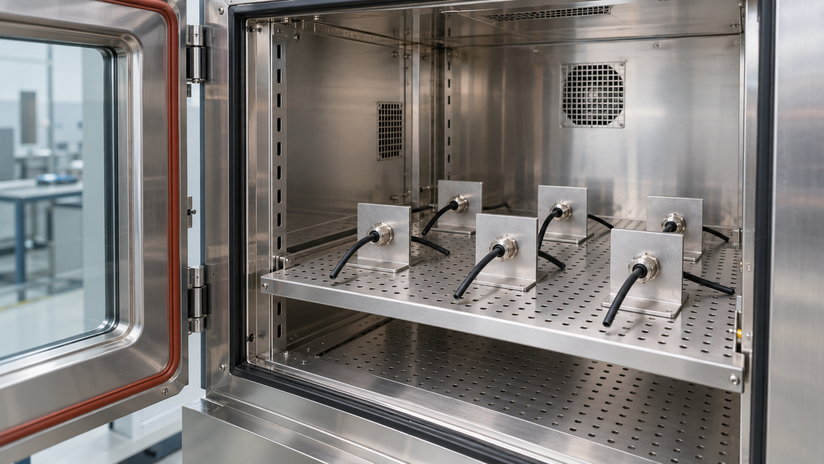
<p><strong>母體</strong>是此結果預計描述的一組組件。固定電纜密封接頭設計、密封膠料、電纜外被與直徑、安裝配置及安裝狀態。若批次或型號有所不同，應保留其識別資訊，以便檢查其影響，而非透過合併資料將差異掩蓋。</p>
<p>開始暴露前先選定功能性失效判定端點。超過定義門檻的洩漏、保持力喪失與可見塗層損傷，是不同的事件，可能形成不同的壽命分布。我會選擇符合工程決策的事件，再定義量測方法與門檻，讓每個試樣都依一致標準判定。</p>
<p><a href="/zh-hant/blog/the-physics-of-water-ingress-how-seals-fail-and-how-to-prevent-it/">進水失效指南</a>有助區分電纜密封處與安裝介面的洩漏路徑。即使兩者都會使水進入外殼，也可能需要不同的檢查方式。</p>
<p>分析時應使用同一個暴露計時基準：運轉小時、經過的環境暴露時間或計數循環。指定起算時間及暫停時的處理方式。本文所討論的壽命是未經修復組件首次失效的時間。修復後再次失效則需要能描述修復與再發情況的模型及資料結構。</p>
<figure>
<img alt="分開直立的電纜引入試片，各自帶有黑色電纜尾端，間隔排列在箱門打開的環境試驗箱內的架上。" src="/images/blog/weibull-cable-entry-reliability/weibull-cable-entry-reliability-scene-01.png" width="1672" height="941" loading="lazy" decoding="async">
<figcaption>各自裝有電纜密封接頭與電纜尾端的引入口試樣，彼此分開安放在試驗箱架上。</figcaption>
</figure>
<p>隨機抽樣或以其他合理方式取得的樣本，應能代表所討論的母體。退回的元件有助於診斷，但只看退回品的清單會漏掉已安裝且仍存活的單位。應將失效紀錄與仍在觀察中的單位及其暴露歷程連結。<a href="/zh-hant/blog/cable-gland-durability-testing-a-head-to-head-comparison-simulating-10-years-of-industrial-use/">耐久性試驗指南</a>說明組件界定與暴露規劃如何配合。</p>
<h2 id="keep-exact-failures-and-censored-records-distinct">區分確切失效與設限紀錄</h2>
<p><strong>右設限</strong>表示單位在最後一次觀察時仍未發生定義的失效，但其後的失效時間未知。<strong>區間設限</strong>表示事件發生在兩次觀察時間之間。<a href="https://www.itl.nist.gov/div898/handbook/apr/section1/apr131.htm">NIST 的設限說明</a>解釋這些資料類型，以及為何都應納入分析。</p>
<p>使用以下六個試樣的假設資料集。假設試樣壽命彼此獨立且來自相同母體、暴露條件一致、持續監測判定端點，並事先規劃在 300 h 停止試驗。</p>
<table>
<thead>
<tr>
<th>試樣</th>
<th style="text-align: right">觀察時間</th>
<th>狀態</th>
<th>意義</th>
</tr>
</thead>
<tbody>
<tr>
<td>A</td>
<td style="text-align: right">100 h</td>
<td>失效</td>
<td>符合既定失效準則的失效首次發生於 100 h</td>
</tr>
<tr>
<td>B</td>
<td style="text-align: right">180 h</td>
<td>失效</td>
<td>符合既定失效準則的失效首次發生於 180 h</td>
</tr>
<tr>
<td>C</td>
<td style="text-align: right">260 h</td>
<td>失效</td>
<td>符合既定失效準則的失效首次發生於 260 h</td>
</tr>
<tr>
<td>D</td>
<td style="text-align: right">300 h</td>
<td>右設限</td>
<td>存活至試驗端點</td>
</tr>
<tr>
<td>E</td>
<td style="text-align: right">300 h</td>
<td>右設限</td>
<td>存活至試驗端點</td>
</tr>
<tr>
<td>F</td>
<td style="text-align: right">300 h</td>
<td>右設限</td>
<td>存活至試驗端點</td>
</tr>
</tbody>
</table>
<p>狀態欄位應獨立記錄。300 h 的三筆資料是存活觀測，其貢獻不同於在 300 h 記錄的失效。刪除這些資料會漏掉樣本中仍存活的一半；將它們改記為失效則會改變實際發生的情況。</p>
<p>若定期檢查判定端點，應記錄最後一次通過及首次失敗的時間。若在 200 h 通過檢查，並於 250 h 失敗，則事件時間落在該區間。應使用能處理區間設限的配適方法，不要指定區間中點或檢查時間作為確切事件時間。</p>
<p>我也會保留每筆觀測結束的原因。事先規劃的停止，與因試樣看似接近失效而將其移出試驗，支持不同的設限假設。選擇分析方法前，應調查這類移除及其與壽命的關係。</p>
<h2 id="fit-the-observations-and-check-the-model">配適觀測資料並檢查模型</h2>
<p><strong>最大概似估計</strong>（MLE）會選擇一組參數，使記錄的觀測資料與所選分布最一致。確切失效在其失效時間提供機率密度；右設限單位則依其觀察時間提供存活機率。區間觀測會提供事件發生於兩次讀值之間的機率。<a href="https://www.itl.nist.gov/div898/handbook/apr/section4/apr412.htm">NIST 的 MLE 說明</a>列出這些不同的概似項。</p>
<h3 id="worked-example-changing-the-status-changes-the-result">範例：狀態編碼方式會改變結果</h3>
<p>以上六筆假設紀錄以位置固定為零的兩參數威布爾最大概似估計計算，形狀約為 2.047、尺度為 353.7 h，B10 為 117.8 h。下表將此結果與兩種刻意錯誤處理相同資料的方式比較。</p>
<table>
<thead>
<tr>
<th>處理方式</th>
<th style="text-align: right">形狀估計值</th>
<th style="text-align: right">尺度估計值</th>
<th style="text-align: right">B10 估計值</th>
<th>對資料的影響</th>
</tr>
</thead>
<tbody>
<tr>
<td>三筆失效加上三筆右設限存活資料</td>
<td style="text-align: right">2.047</td>
<td style="text-align: right">353.7 h</td>
<td style="text-align: right">117.8 h</td>
<td>保留所述觀測資料</td>
</tr>
<tr>
<td>刪除三筆存活資料</td>
<td style="text-align: right">3.121</td>
<td style="text-align: right">202.2 h</td>
<td style="text-align: right">98.3 h</td>
<td>只配適失效子集</td>
</tr>
<tr>
<td>將三筆 300 h 存活資料都標記為失效</td>
<td style="text-align: right">4.016</td>
<td style="text-align: right">266.0 h</td>
<td style="text-align: right">151.9 h</td>
<td>加入範例中不存在的事件</td>
</tr>
</tbody>
</table>
<p>我發現，在這組假設資料中，將存活資料改記為失效會提高 B10：從 117.8 h 增至 151.9 h。刪除相同的存活資料則會使 B10 降至 98.3 h。這兩種相反的影響，表示匯入報告時應優先核對狀態欄位；編碼錯誤可能讓結果朝任一方向偏移。先使用正確狀態，再評估配適情形與不確定性。只有三筆觀測到的失效時，形狀與下尾估計都很敏感。若要進行有力的工程比較，還需要資訊量更充分的暴露資料與信賴度分析。</p>
<p><strong>機率圖</strong>會在轉換後的座標軸上比較觀測資料與模型；這與前述一般累積曲線不同。<a href="https://www.itl.nist.gov/div898/handbook/apr/section2/apr221.htm">NIST 的機率繪圖方法</a>會在繪圖位置中納入設限資料的處理。若資料大致呈線性，表示其與所選模型相符。</p>
<p>調查曲線彎曲、批次群聚、早期離群值及試樣位置效應。除非有記錄明確的量測或母體理由，否則應保留每筆資料。使用相同觀測值比較合理的分布。NIST 的<a href="https://www.itl.nist.gov/div898/handbook/apr/section4/apr413.htm">威布爾範例</a>比較配適統計量相近的威布爾與對數常態模型，說明僅憑曲線外觀平順，仍不足以確定模型選擇。</p>
<p>失效機制也可能互相競爭。若腐蝕在洩漏失效發生前就使觀察結束，應同時記錄導致觀察結束的事件，以及洩漏時間的設限資料。<a href="https://www.itl.nist.gov/div898/handbook/apr/section1/apr181.htm">NIST 的競爭風險模型</a>在機制彼此獨立並以首次失效為前提下，合併不同機制。若接合處移動同時促進腐蝕與洩漏，選擇模型時應調查這項共同原因。</p>
<h2 id="read-the-confidence-bound-beside-the-life-estimate">在壽命估計旁查看信賴界限</h2>
<p><strong>信賴界限</strong>表示在分析假設下，對所估計母體量值的不確定性。B10 的下側信賴界限回答的問題不同於 B10 點估計值。應將信賴水準、單側或雙側形式及計算方法與數值一併記錄。</p>
<p>例如，假設要求 B10 的單側 95% 下側信賴界限至少為 1,000 h。某假設報告的 B10 點估計值為 1,300 h，但其下側界限為 900 h，因此未達要求。點估計值高出 300 h，無法補足所要求界限短少的 100 h。</p>
<p>我會一併查看樣本數與失效數。信賴區間描述估計百分位數或參數的不確定性；這不同於涵蓋該比例個別壽命的區間。比較報告時，應採用相同的壽命指標、信賴慣例、判定端點及暴露基準。</p>
<p>若沒有失效，應報告存活單位數及其存活時間。在未施加參數約束的兩參數威布爾配適中，提高尺度可使全數存活資料的概似持續增加，因此僅憑這些觀測無法確定有限的形狀與尺度估計值。另行指定的可靠度證明方法，則可在其明列假設下使用這些存活結果。</p>
<p>實用的解讀順序是先確認壽命指標，再檢查觀測與設限資料、模型配適情形，最後比較要求的信賴界限。接著針對左右決策的因素追查：暴露時間、失效數、混合母體或不確定的機制。</p>
<h2 id="connect-accelerated-test-life-to-service-conditions">將加速試驗壽命連結至服務條件</h2>
<p>在較高應力下配適的威布爾曲線描述的是該應力條件。若要推估正常使用情況，須將壽命分布與相關失效機制的加速關係結合。<a href="https://www.itl.nist.gov/div898/handbook/apr/section4/apr43.htm">NIST 的使用條件推估說明</a>解釋為何兩個模型都很重要，尤其當服務預測落在觀測資料稀少的早期尾端時。</p>
<p>確認加速試驗與服務條件下的失效機制相同。較高溫度可能改變密封件的劣化機制；濕氣、化學品與移動也可能以不同方式影響組件。應將應力歷程視為模型的一部分，不要把無關的時數合併成單一累積年限。<a href="/zh-hant/blog/how-does-environmental-aging-affect-cable-gland-seal-performance-over-time/">密封件老化指南</a>說明這些應力與密封功能的關聯。</p>
<p>我會尋找較低應力、較長時間或現場觀測資料，以檢查推估在接近預定使用條件時是否合理。保留以原始小時或循環表示的試驗條件估計值，並為服務壽命推估說明使用條件組合。如此一來，B10 數值在納入維護或設計決策時，仍會連結至特定母體、失效事件及暴露模型。</p>
<h2 id="conclusion">結論</h2>
<p>B10、特徵壽命與平均壽命描述威布爾壽命模型的不同部分。相同的特徵壽命可能掩蓋差異很大的早期失效行為，因此應比較符合預定暴露條件與決策需求的指標。分析時要依正確狀態納入失效與存活試樣。</p>
<p>我會在點估計值旁查看信賴界限，再檢查母體、失效定義及應力條件。範例顯示這些細節會如何改變數值結果。推估服務壽命時，應先將試驗模型連結至實際機制及使用條件組合，再將結果用於維護或設計決策。</p>
<h2 id="faq-about-weibull-reliability-analysis">威布爾可靠度分析常見問題</h2>
<h3 id="is-weibull-characteristic-life-the-average-life">威布爾特徵壽命就是平均壽命嗎？</h3>
<p>特徵壽命是尺度值；在兩參數模型中，該值對應約 63.2% 的累積失效機率。平均壽命取決於形狀與尺度，是不同的量。比較期間前，先確認報告所稱的壽命指標；B10 著重較早出現的第十百分位失效暴露量。</p>
<h3 id="how-should-specimens-that-survive-the-test-be-recorded">試驗中存活的試樣應如何記錄？</h3>
<p>保留最後觀察時間、右設限狀態，以及觀察結束的原因。這些紀錄表示試樣存活至該時間，並會納入壽命分析。使用可處理設限資料的分析方法。若在定期檢查時發現失效，應保留最後一次通過與首次失敗所界定的區間，不要指定一個精確事件時間。</p>
<h3 id="what-does-b10-say-about-individual-cable-entries">B10 對個別電纜引入口代表什麼？</h3>
<p>B10 是模型中累積失效機率達 10% 時的暴露量，在定義條件下相當於 90% 存活率。有些單位較早失效，有些則較晚。此估計也有不確定性，因此判斷可靠度目標時，應比較所要求的信賴界限。維護規劃還會考量失效後果及使用條件組合。</p>
<h3 id="how-can-an-accelerated-weibull-curve-support-a-service-life-prediction">加速威布爾曲線如何支援使用壽命預測？</h3>
<p>將壽命分布與相關失效機制及使用條件所適用的加速關係結合。確認該機制仍適用，並以適當的較低應力、較長時間或現場觀測比較推估結果。解讀推估壽命時，應明確說明母體、失效判定條件、暴露計時基準及不確定性。</p>
<h3 id="sources-and-technical-references">來源與技術參考資料</h3>
<ul>
<li><a href="https://webstore.iec.ch/en/publication/5698">IEC 61649:2008 — 威布爾分析</a>，查閱日期：2026-10-29。</li>
<li><a href="https://www.itl.nist.gov/div898/handbook/apr/section1/apr131.htm">NIST — 設限資料</a>，查閱日期：2026-10-29。</li>
<li><a href="https://www.itl.nist.gov/div898/handbook/apr/section1/apr162.htm">NIST — 威布爾壽命模型</a>，查閱日期：2026-10-29。</li>
<li><a href="https://www.itl.nist.gov/div898/handbook/eda/section3/eda3668.htm">NIST — 威布爾分布與分位數</a>，查閱日期：2026-10-29。</li>
<li><a href="https://www.itl.nist.gov/div898/handbook/apr/section4/apr412.htm">NIST — 最大概似估計</a>，查閱日期：2026-10-29。</li>
<li><a href="https://www.itl.nist.gov/div898/handbook/apr/section2/apr221.htm">NIST — 機率繪圖</a>，查閱日期：2026-10-29。</li>
<li><a href="https://www.itl.nist.gov/div898/handbook/apr/section1/apr181.htm">NIST — 競爭風險模型</a>，查閱日期：2026-10-29。</li>
<li><a href="https://www.itl.nist.gov/div898/handbook/apr/section4/apr413.htm">NIST — 威布爾最大概似估計範例</a>，查閱日期：2026-10-29。</li>
<li><a href="https://www.itl.nist.gov/div898/handbook/apr/section4/apr43.htm">NIST — 推估使用條件下的可靠度</a>，查閱日期：2026-10-29。</li>
</ul>
